In order to assess the model performance on a given dataset, we need to measure how closely its predictions align with the actual data. In regression settings, we often use mean squared error (MSE) and a smaller MSE means the predicted responses are closer to the true responses.
While we can get MSE from both training and the test data, what we really care is the model performance on unseen test data. This is where the bias-variance tradeoff comes into play. The process of selecting a model that minimizes MSE on the test data inherently involves a tradeoff between bias and variance. In this blog post, we will explore the concept of the bias-variance tradeoff with the help of visual aids and a mathematical proof.
Bias refers to the error that results from oversimplifying the model. A model with high bias may be too simple to capture the complexity of the underlying data or identify the relationship between input and outcome variables.
On the other side, variance refers to the amount by which the model would change if we estimated it using a different training set. A model with high variance means that the model is overly complex such that it captures noises in the data instead of the underlying patterns. This leads to the problem of over-fitting where our model performs too well on the training data but poorly on unseen data.
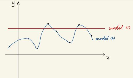
As shown in the following graph, model (1) which is a constant has extremely high bias but zero variance, while model (2) which looks extremely wiggly by just connecting observed data points has low bias but high variance.
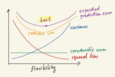
The bias-variance tradeoff arises because as the flexibility (or complexity) of the model increases, we often have smaller bias but larger variance, and vice versa. The relative changes in bias and variance determine whether the test MSE increases or decreases.
Mathematically, we can decompose expected prediction error (expected test MSE) into two components: irreducible error and reducible error. Irreducible error is the variation that cannot be reduced by modifying the model, and is associated with unmeasured variables. Reducible error is comprised of the sum of squared bias and variance of the model. Our objective is to minimize reducible error while recognizing that we cannot surpass the irreducible error. A proof of this decomposition can be found at the end of this post.
The following graph contains all the concepts we’ve discussed in this post. In future posts, we will delve deeper into how to find an optimal balance between bias and variance using different machine learning models.
Proof
Suppose that we have a simple model specified below, we can break down the expected prediction error (expected test MSE) \(E(y_0) - \hat f(x_0))^2\) and see where the bias-variance tradeoff comes from.
\[ y = f(x) + \epsilon \\ \text{where } E(\epsilon) = 0, \epsilon \perp x, x \text{ is fixed } \]
We can rewrite the expected prediction error as below \[ E(y_0) - \hat f(x_0))^2 \\ = E(y_0 \color{red}{- f(x_0) + f(x_0)} \color{blue}{- E\hat f(x_0) + E\hat f(X_0)} - \hat f(x_0))^2 \] What’s within \(E()^2\) can be thought of as a summation of three parts a, b, and c where \[ a = y_0 - f(x_0) \\ b = f(x_0) - E\hat f(x_0) \\ c = E\hat f(x_0) - \hat f(x_0) \] Recall that \[ (a+b+c)^2 = a^2 + b^2 + c^2 + 2ab + 2bc + 2ac \] then we have \[ E(y_0) - \hat f(x_0))^2 \\ = E(a^2) + E(b^2) + E(c^2) + 2E(ab) + 2E(bc) + 2E(ac) \] Let’s walk through the last three terms first.
It’s not hard to see \(E(ab) = 0\), \(E(bc)=0\), and \(E(ac)=0\) as highlighted below.
\[ \begin{aligned} E(ab) &= E((y_0 - f(x_0))(f(x_0) - E \hat f(x_0))) \\ &= \color{red}{E(y_0 - f(x_0))}(f(x_0) - E \hat f(x_0))\\ &= 0 \end{aligned} \]
\[ \begin{aligned} E(bc) &= (f(x_0) - E \hat f(x_0)) E((E\hat f(x_0) - \hat f(x_0)))\\ &= (f(x_0) - E \hat f(x_0)) \color{red}{(E \hat f(x_0) - E \hat f(x_0))} \\ &= 0 \end{aligned} \] \[ \begin{aligned} E(ac) &= E((y_0) - f(x_0)) \color{red}{(E \hat f(x_0) - \hat f(x_0))}\\ &= 0 \end{aligned} \] Now, let’s turn to the first three terms.
Recall that \[ E(E(\hat \theta) - \hat \theta)^2 = var(\hat \theta)\\ \text{Bias}(\hat \theta)^2 = (E(\hat \theta) - \theta))^2 \]
We can rewrite these terms as follows: \[ \begin{aligned} E(a^2) &= E(y_0 - f(x_0))^2 \\ &= E(\epsilon_0)^2 \\ &= E(\epsilon^2) - \color{red}{(E(\epsilon))^2} \\ &= var(\epsilon) \end{aligned} \]
\[ \begin{aligned} E(b^2) &= E(f(x_0) - E \hat f(x_0))^2 \\ &= (f(x_0) - E \hat f(x_0))^2 \\ &= \text{Bias}^2(\hat f(x_0)) \end{aligned} \] \[ \begin{aligned} E(c^2) &= E(E\hat f(x_0) - \hat f(x_0))^2 \\ &= var(\hat f(x_0)) \end{aligned} \] Taken together, it becomes clear that the expected prediction error can be decomposed into three parts. The first term \(var(\epsilon)\) is the irreducible error and the others constitute the reducible error that we try to minimize.
\[ E(y_0) - \hat f(x_0))^2 = \color{red}{var(\epsilon)} + \color{blue}{\text{Bias}^2(\hat f(x_0)) + var(\hat f(x_0))} \]